Activity Landscape Plotter V.1

DIFACQUIM

Welcome to this first online Activity Landscape Plotter. Here you will be able to perform analyses of activity landscape using Structure-Activity Similarity (SAS) maps, Dual Activity-Difference (DAD) maps and other metrics.

If you use this app please cite this reference:

Gonzalez-Medina M, Mendez-Lucio O, Medina-Franco JL. Activity Landscape Plotter: A Web-based Application for the Analysis of Structure-Activity Relationships. J Chem Inf Model (2017) 57(3), 397-402.

This App was developed by Mariana Gonzalez-Medina Oscar Mendez-Lucio and Jose L. Medina-Franco members of DIFACQUIM The group is based in the Pharmacy Department of the School of Chemistry in Universidad Nacional Autonoma de Mexico.

Last update July, 2017

What are they for?

Structure-Activity Similarity (SAS) maps.

SAS maps were introuced to find a relationship between structure and activity, based on a systematic pairwise comparison of all the compounds in a data set. You can find more information here.

With this App you can automatically obtain all the information required to generate and analyze SAS maps using your own activity data for one or more biological targets. You can customize the SAS maps and download the raw data as described in the Instructions.

Dual Activity-Difference (DAD) maps.

DAD maps depict pairwise activity differences for each possible pair of compounds in a data set against two targets. These maps are helpful to differentiate when a strucutural modification increases or decreases the activity for one target or the other. You can find more information here.

With this App you can automatically obtain all the information required to plot and analyze DAD maps, using the biological activities in your input file. You can customize the DAD maps and download the raw data as described in the Instructions.

Must of the errors occur beacause your input file does not have the right format. See the template if you are not sure about the format.

1. How to introduce your data:

You will need a comma delimited file with these columns:

First column: SMILES, do not leave empty rows

Second column: first activity, it is okay if you leave empty rows in this column

Third column: second activity, same as for the second column. If you do not have more than one activity leave the rest of the activity columns empty

Fourth column: third activity, leave this column empty if you do not have a third activity

Fifth column: Same as for the fourth and third columns

Sixth column: this column is for your compounds IDs, make sure the last column in your file has the IDs.

You have to introduce your activity data as PIC50 =-log10(IC50) or pkI=-log10(kI50).

You can download the template from the template tab.

2. After you upload your data, a plot with the pre-stablished settings on the App will appear. This could take a few seconds if you are analyzing many compounds. Wait until the first plot appears before you start changing the settings.

3. You can choose a fingerpirnt, the column with activity and adjust the thresholds.

4. You can choose how to color the data points (the most active compound in the pair, SALI value, selectivity or similarity).

5. Whenever you change an input, wait until the plot is completely loaded before you download new data.

Information about each plot and the metrics used.

SAS map.

X axis or structural similarity.

For the SAS maps you can choose the fingerprint you want to use (ECFP, PubChem, MACCS keys). These fingerprints are calculated using the R package called rcdk. More information on this package and fingerprints can be found here. For topological fingerprints, like ECFP, you can choose if you want to use a diameter of 4 or 6. The structural similarity plotted on the X axis is computed using the fingerprint of your choice and Tanimoto similarity.

Y axis or activity difference.

The activity difference plotted on the Y axis is the absolute difference between the activity values of each pair of compounds.

Thresholds and areas of the plot.

You can change the X and Y axis thresholds. Depending on tese thresholds the number of compounds that you will download from each area in the plot will change.

Your SAS map will be divided in 4 areas:

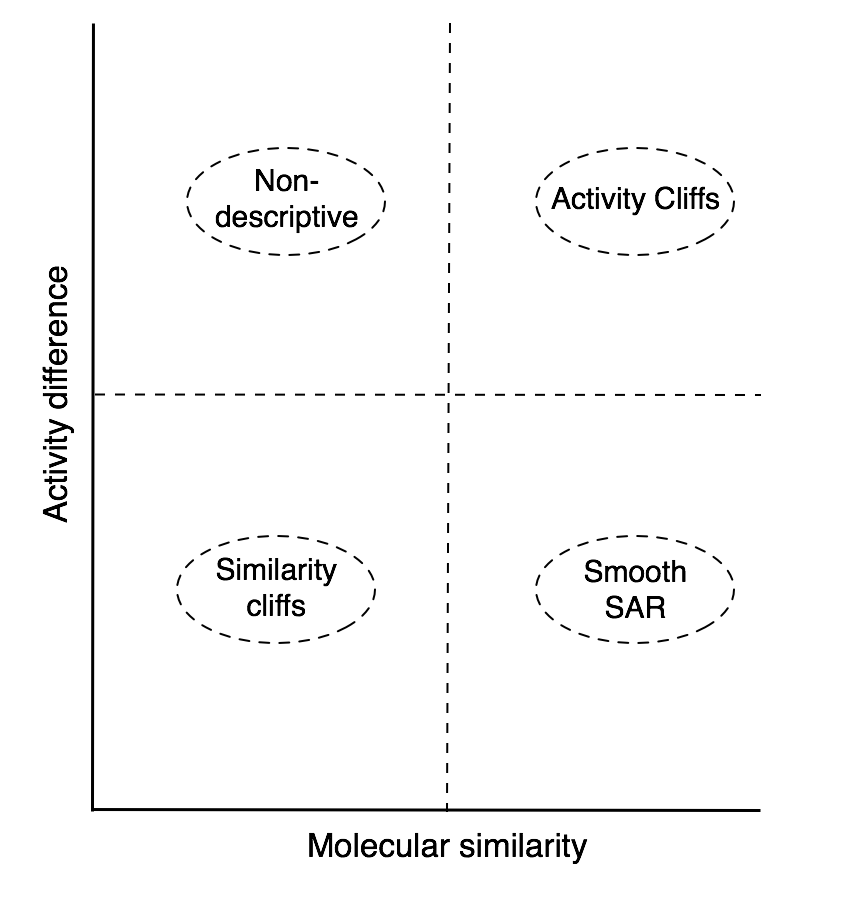
1. The bottom left area contains pairs of compounds that have low molecular similarity and low activity difference, i.e., similarity cliffs.

2. In the bottom right area, or smooth SAR, you can find pairs of compounds that have high molecular similarity and low activity difference.

3. The top right area contains activity cliffs i.e., pairs of compounds with high molecular similarity and high activity difference.

4. The top left area or non-descriptive, contains pairs of compounds that have low structural similarity and high activity difference.

You can download all the data generated to plot the SAS map and the information for all the pairs of compounds on each area of the plot, as well as their similarity, the most active compound in the pair, activity difference and SALI If you change a certain setting you will have to wait until the new is produced before you can download the new data.

If you select a dot or group of dots on the plot, it will tell you which pair or pairs of compounds are in that area.

The color of the plot changes depending on the values calculated for the Structure-Activity Landscape Index (SALI) and the most active compound in the pair. You can find more information on SALI here. Pairs of compounds with the highest SALI will be colored green, pairs of compounds with intermediate SALI values will be orange to yellow and pairs of compounds in red will have the lowest SALI values. Similarly to SALI the most active compounds on each pair will be red, intermediate compounds will be yellow-to-orange and the less active will be green. You can find some examples of SAS maps color-coded by the most active compound in the pair here.

DAD maps.

X and Y axis Activity Difference 1 and Activity Difference 2.

For the DAD map you can choose two biological activities from your input file to be plotted. Each point on the plot corresponds to the pairwise activity difference against target one (activity difference 1) and the pairwise activity difference agains target 2 (activity difference 2) for each possible pair in the data set.

Thresholds and areas on the plot.

You can change the X and Y axis superior and inferior thresholds. Depending on these thresholds the number of compounds that you will download from each area in the plot will change.

Your DAD map will be divided in 9 areas:

1. Areas Z1 up and Z1 down or Z1u and Z1d, respectively, contain pairs of compounds for which structural changes have a similar impact on the activity towards the two targets. For Z1d the structural changes decrease the activity for the two targets and for Z1u the structural changes increase the activity for the two targets.

2. Areas Z2 up and Z2 down or Z2u and Z2d, respectively: indicate that the change in activity for the compounds in the pair is opposite for each target, i.e., changes in structure increase the activity for one target, while decreasing activity for the other target. For Z2u, structural changes increased the activity on the second target and decreased the activity in the first target. Z2d, structural changes decrease the activity for the second target and increase the activity for the first target.

3. Areas Z3 and Z4 or Z3d, Z3u and Z4l, Z4r: indicate that structural changes result in significant changes in activity towards one target, but not a large change towards the other target.

4. 4. Area Z5 indicates pair of compounds with similar activity against target one and target 2, therefore, structural changes have little or no impact on the activity against the two targets. Compounds in Z5 might be of significant interest if the goal of the analysis is to identify promiscuous hits.

The classification of data points in an activity-difference map is independent of the structure similarity. However, in the DAD map the structural similarity of each pair of compounds can be mapped using a continuous color scale: compounds with high similarity will be colored green, compounds with intermediate similarity will be colored yellow to orange and compounds with low similarity will be red. You can also add color to the data points with the selectivity option. For this option, if a data point is colored red this indicates that one of the compounds in that pair could be selective to one of the targets; yellow to orange, one of compounds is moderately selective; green, there are no important activity differences.

You can download all the data used to plot the DAD map and the information for all the pairs of compounds on each area of the plot, as well as their selectivity, similarity, activity difference 1 and activity difference 2. If you change a certain setting you will have to wait until the new plot is produced before you can download the new data.

If you select a data point or a group of data points on the plot, it will tell you which pair or pairs of compounds are in that area.

You can find more information about SAS and DAD maps here.